Interpret output from regression analysis
How to interpret the results from a regression analysis? It depends on the question, theory, data quality, and more. But we also need to understand the numbers that Stata produces in the output. In this post we will look closer at them.
Below are the results from an analysis from an American survey conducted in 2018. The dependent variable is how much the respondent earns in a year, in US dollars. The independent variable is how many hours the respondent worked last week. In the real survey there are thousands of responses, but here I randomly selected 46 of them to make the results a little bit easier to show.
| Letter | Meaning |
|---|---|
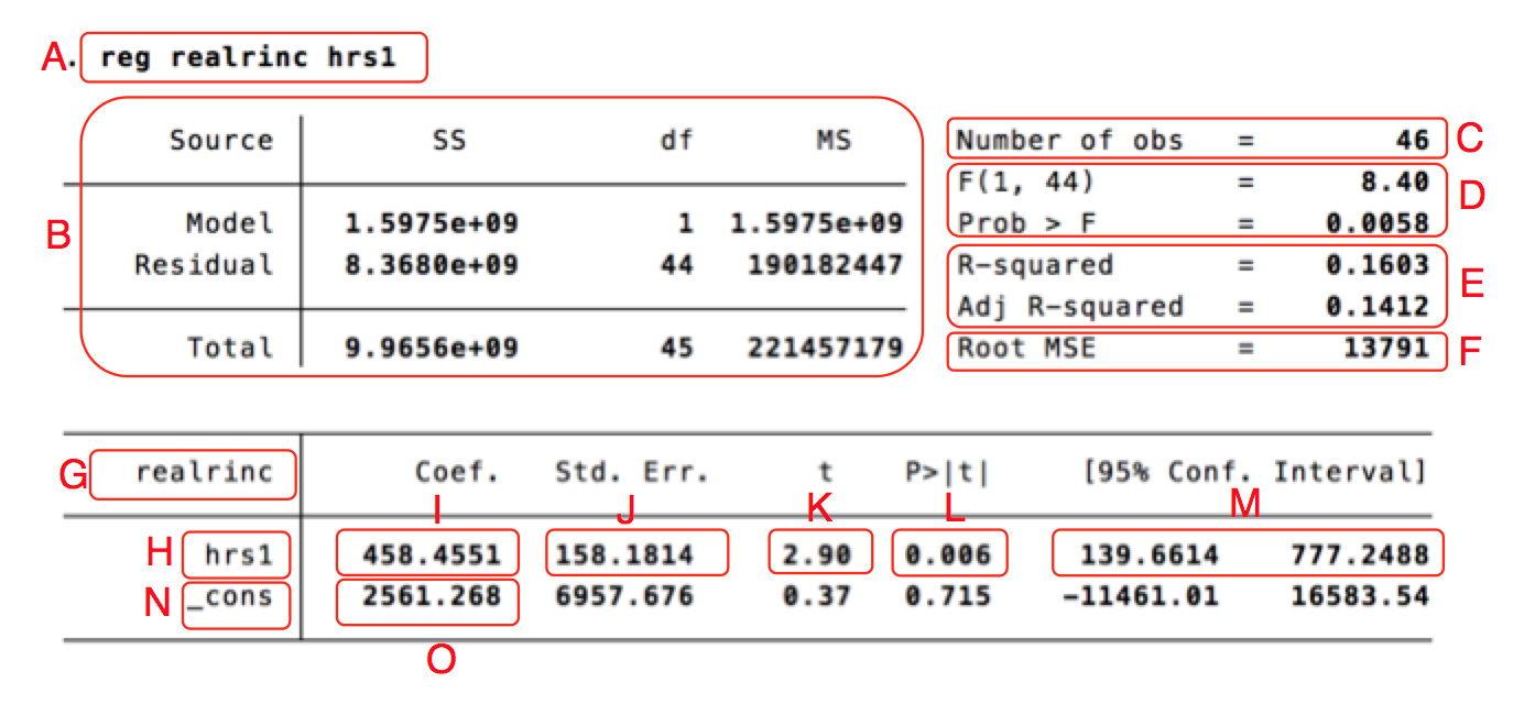
| A | A copy of the regression command that produced the analysis. |
| B | Summaries of values that are used to calculate other values in the analysis. This part is rarely interpreted or reported in papers. |
| C | The number of observations in the analysis: 46. Also called the n-value. |
| D | THe F-value (8.40). It is measure of the entire model, used to test the hypothesis that any of the independent variables in the model has an effect on the dependent variable. We also get a significance test for the F-value (Prob > F). In this case the F-value is significant on the 99 percent level, since the significance value is below 0.01. We thus have good reason to believe that at least one of the independent variables has an effect (we only have one independent variable in this model). |
| E | The $R^2$ value, which shows the proportion explained variance. In other words, how much of the variation in the dependent variable that can be attributed to variation in the independent variable. More explicitly, how much of the variation in people's earnings can be explained by variation in how much people work? In this case te value is 0.1603 which usually is expressed as "16 percent of the variation in income is explained by the variation in working hours." We can also see the "adjusted R-square" value, which is an adjusted version of $R^2$ value. The normal measure can only rise when we add independent variables to the model, even though the variables might lack explanatory power. The adjusted value instead gets a "penalty" for each new variable. The value therefore only goes up when the independent variable adds explanatory power, which makes the measure more useful when comparing models. |
| F | "Root Mean Square Error", a measure of how close the model's predictions are to reality; a typical error. In this case: 13791 dollars. It basically captures something similar to the $R^2$ value, but expressed in the scale of the dependent variable. We can therefore not use it to compared analyses with different dependent variables with each other. |
| G | The name of the dependent variable, "realrinc". |
| H | The name of the independent variable, "hrs1". If we have more independent variables they get one row each. |
| I | The b-coefficient for "hrs1", 458.4551. It means that if we increase hrs1 by one step (work one hour more each week) the yearly income is expected to rise with 458.4551 dollars. |
| J | The standard error for the b-coefficient for hrs1, a measure of the uncertainty of the estimate. The larger the standard error is in relation to the b-coefficient, the less certain we can be that the coefficient is in the population (the american people, in this case). |
| K | The t-value for hrs1. It shows how improbable it is that we would get a relationship this strong between hrs1 and realrinc, had there been none in the population. It is obtained by dividing the b-coefficient with the standard error. The higher the t-value (or more accurately, the further from zero. It can also be negative), the more improbable. If it is very improbable, the natural conclusion is that there actually is a relationship between hous worked and income, also in the population. |
| L | The p-value, or the significance value. It basically shows the same thing as the t-value, but expressed slightly differently. It shows how often we get a relationship this strong between hrs1 and realrinc, even if there is none in the population, simply due to chance in the sampling. In this case the value is 0.006, which means that even if there is no relationship between working hours and income in the population, we would get a relationship this strong 6 times out of 1000, if we made random samples of 46 people. The normal decision criteria is 0.05 - if the p-value is below 0.05 we say that the result is statistically significant on the 95 percent level. We then draw the conclusion that there is a relationship between the variables in the population. |
| M | The confidence interval for the b-coefficient for hrs1. The standard error shows that there is some uncertainty around the estimate. The confidence interval shows the same thing, but in an easy way. We can not be sure that the b-coefficient is exactly 458, but we can be pretty sure that is is something between 139.66 and 777.25. The 95 percent confidence interval is constructed so that if we repeat the sample a 100 times, the confidence interval will cover the true value 95 times out of 100. If the confidence interval does not cover 0, the p-value is always below 0.05. |
| N | The name for the intercept, the value we expect the dependent variable to have when all the independent variables in the model are zero - in this case for people who did not work last week. |
| O | The value of the intercept. The people in the survey that do not work at all are expected to earn 2561 dollars per year, on average. |
The other values on the row of the intercept mean the same thing for the intercept as they did for the b-coefficient for hrs1. But they are seldom of theoretical interest and are rarely interpreted.
Note that the standard error, t-value, p-value and confidence interval all deal with the same thing: uncertainty of the estimate. Generally we only mention one when we discuss the results. If the standard error is small in relation to the b-coefficient, the t-value will be high, the p-value will be low, and the confidence interval will be small.
A graphical comparison
We can also have a look at a scatterplot that shows the regression analaysis. Some of the things we saw in the output can also be seen in the graph, and are denoted with the same letters:
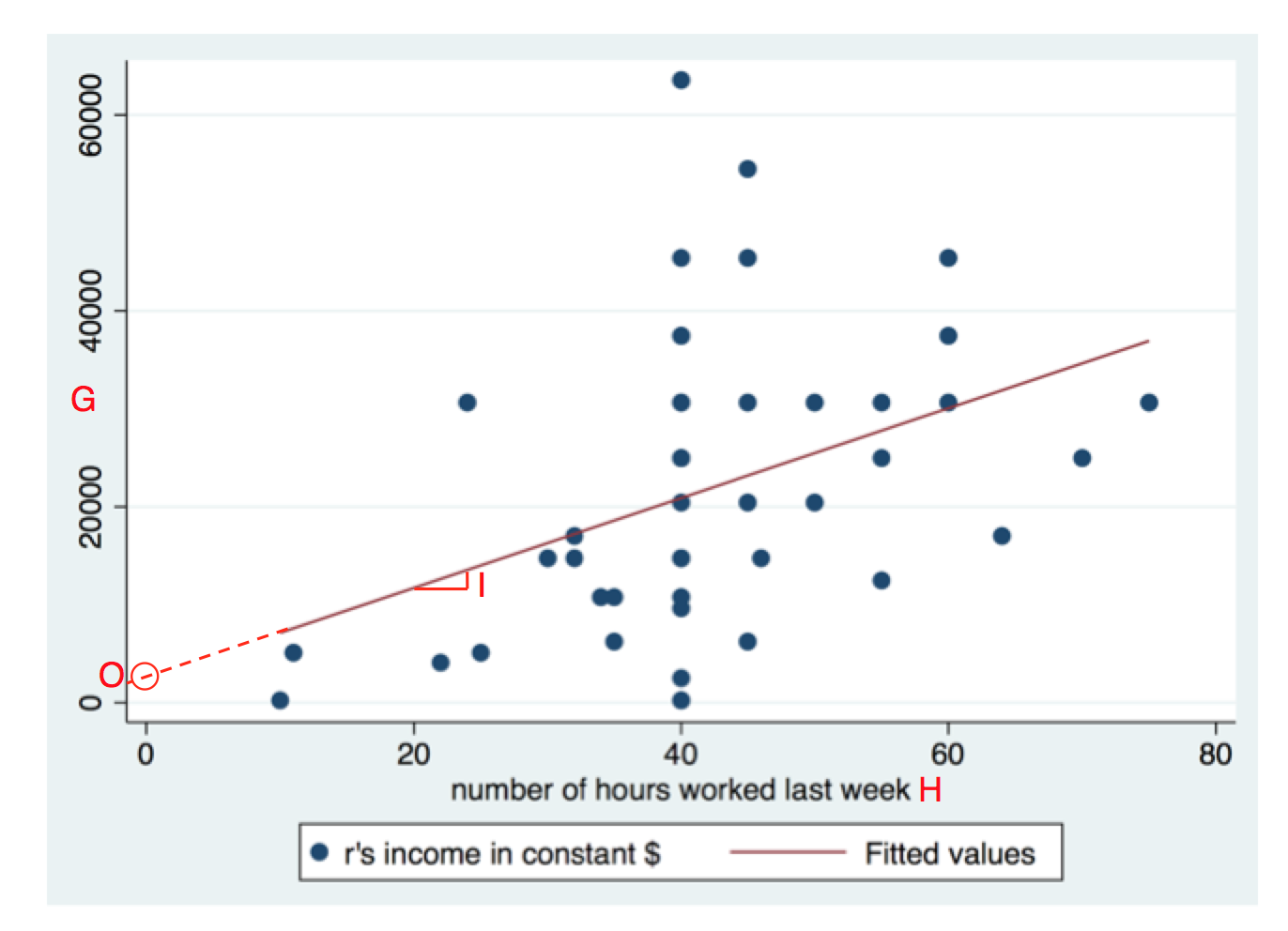
On the Y axis we have G, the dependent variable. The independent variable hrs1 is found on the X axis, denoted with an H. Each person is a dot (there is fewer than 46 dots, since several persons have identical values, and thus overlap).
The b-coefficient for hrs1 was denoted with an I in the table, and is here shown as the slope of the regression line. When we take a step to the right we end up 458.4551 steps higher up on the Y axis, if we follow the regression line.
The intercept (denoted with a O) ais found where the regression line passes the zero of the X axis. That is, our guess for how much a person who does not work at all will make each year. There were however no such persons in the sample.
The $R^2$ value and the standard error of the b-coefficient are both determined by the spread of the dots around the regression line. The larger the spread, the higher the standard error, and the lower the $R^2$ value.
Conclusion
That is all! When we have more independent variables we can not as directly translate the analysis to a two-dimensional scatterplot, but the principle is the same. The b-coefficients still signify how much we expect the dependent variable to increase when we increase the independent variable one step, but then it is the effect under control for all the other independent variables.