Regression analysis with interaction effects
Regression analysis is used to investigate relationships between variables, with or without control for other vairables. However, in the real world, we often find that relationships are different in different sub-groups of the population, or during different circumstances. The effect of becoming a parent is for instance different among women and men; women see a much larger drop in incomes.
How to account for this in our analyses? One way is to run two separate analyses, one for each group we are interested in (in this case women and men). We then get the effect of becoming a parent among men, and among women.
But we can also do this in one single regression analysis. We then get a sense of how much the effect differs between groups, and also whether the difference in effect is statistically significant. We can then decide whether it is worth the effort to complicate our theoretical model by introducing these separate effects. We can then also hold the effects of all control variables constant. If we run two separate analyses, the control variables would also get different effects in the two models, and that might not be part of our theory.
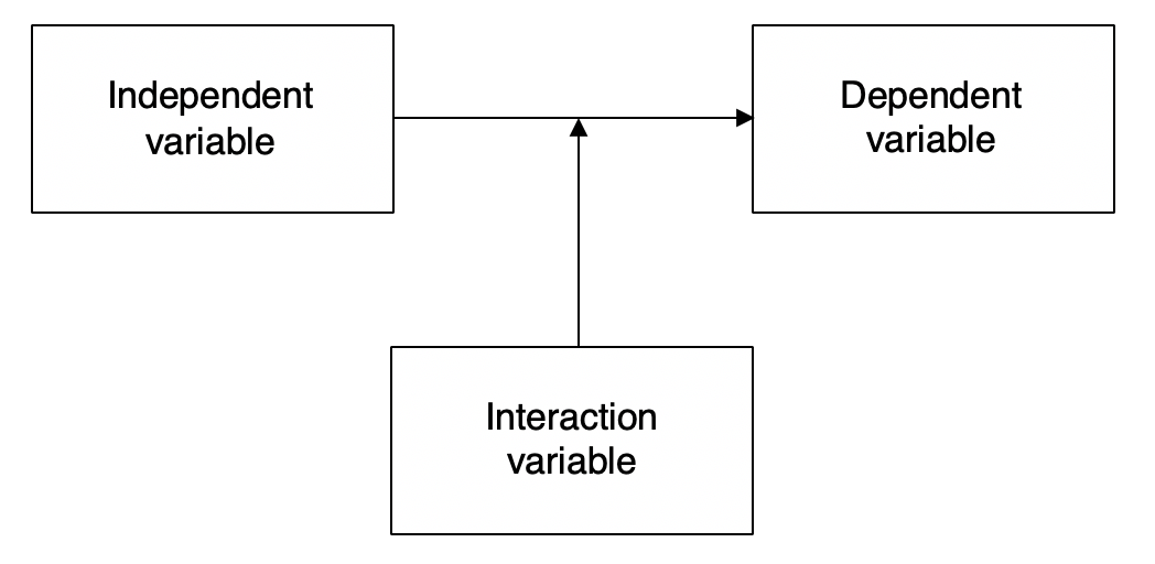
This is called an interaction analysis. It can also be called a moderation analysis, or that we are investigating conditional effects. It means that we let the effect of one variable vary over the values of another variable. It is often graphically represented by a a diagram with an arrow pointing at another arrow. The third variable in this schematic affects the effect of the main independent variable, rather than the value of the independent and dependent variables.
In this guide we will discuss how to do regression analyses where both independent variable and interaction variable only has two values, and how to best present the results.
We will work with data from the american General Social Survey, which is a survey with regular citizens, with questions about a lot of subjects. We will use the 2016 edition. Download the data and put it in your project folder to follow along in the example.
cd "/Users/xsunde/Dropbox/Jupyter/stathelp/data/"
use "GSS2016.dta", clear
Prepare the data for analysis
The question to investigate is the one mentioned above: how becoming a parent affects incomes for women and men. We should really have longitudinal data to properly investigate the question. It would allow us to track individuals before and after they have kids. Since this is cross-sectional data, with information from one point in time, this is not possible. Our conclusions will thus be based on comparisons between parents and non-parents. Of course, this limits our ability to draw conclusions about cause and effect.
We need three variables: gender, income, and number of kids. Information about gender is found in the variable sex where 1 means "male" and 2 "female". To make results more easy to interpret later, we will recode the variable so men have the value 0 and women the value 1. We also rename the variable to "woman" instead of sex. When we increase our variable, it means that the respondent becomes "more woman", metaphorically speaking.
recode sex (1=0) (2=1), generate(woman)
tab woman
We also need a variable for income. There are some to choose from, but the simplest seem to be realrinc, which expresses the respondent's income in dolalrs per year. We can see below that the mean is 23773.
sum realrinc
Finally, we need a variable for the number of kids. There is one that shows exactly that, childs:
tab childs
In this guide we will only compare parents to non-parents, that is the zeros on the varibale to the rest. The largest effects are probably found when you get your first child. Now we create a dummy variable that has the value 0 for respondents without kids, and 1 for respondents with one or more kids. We call it dum_kids.
recode childs (0=0) (1/8 = 1), generate(dum_kids)
tab dum_kids
We now have all the variables we need for the analysis. We can start by doing a correlation matrix that shows how the variables are related, and we also add the variable age, that shows the respondent's age. We will include it as a control variable later on.
pwcorr woman realrinc dum_kids age
The correlation between woman and income is negative, which means that women earn less. More woman = less income. Woman is also positively correlated with having kids. Having kids is in turn positively correlated with incomes - possibly owing to the fact that parents are older, and older people have higher incomes. Age has a positive relationship both with incomes and kids.
Interaction analysis where variables have two values
In the first analysis we will examine how being a parent is related to income, and then redo the analysis for women and men. But first we run a regular regression analysis, without interaction, where we just enter all variables like they are. The dependent variable is income.
reg realrinc woman dum_kids age
Results are as expected. The coefficient for woman is -9748, which means that women in general have 9748 less income (per year) than men, even when controlling for age and having kids.
The coefficient for age is 241, which means that for each extra year of age, the respondents in general have 241 dollars more in yearly income. Being a man does thus has the same effect on income as being $9748/241=40$ years older!
Parents on average have 3603 dollars more in yearly income (when controlling for age and gender).
The effect of having kids is here assumed to be the same for women and men, and we will now investigate whether that is a reasonable assumption. TO do so we need to add what is called an interaction term, a new variable that is the product of woman times dum_kids. Conveniently enough there are automatic functions for doing so in Stata, so we can let Stata create the variable within the analysis. We just add ## between the variables we want to interacti to get the interaction term automatically:
reg realrinc woman##dum_kids age
We now have a new variable in the table, woman#dum_kids. This is the interaction term. We can also note that the coefficients for woman and dum_kids changed a lot. They can now not be interpreted in the same way. The coefficients now show the effect of the variable when the other variable in the interaction is zero. The variable woman shows the difference between women and men that don't have kids. The variable dum_kids shows the difference between parents and non-parents among men.
We need to add the coefficients with the interaction term to calculate what the effects are for the other groups. The interaction term shows how the COEFFICIENTS change when the other variable increases with one unit.
The "effect" of having kids is thus +9213.15 for men. To get the effect for women we need to add the dum_kids coefficient with the interaction term: $9213.15 - 11546.67 * 1 = -2333.52$. This means that mothers have lower incomes than women who are not parents, while fathers have higher income than men who are not parents.
Can we trust this difference in effects? Yes, since the interaction term is significant. It is unlikely that a difference in effects of this size would arise simply because of randomness in the sampling. If the interaction term had been insignificant, it would have been better to trust the simpler model without interaction term, both because it is easier to interpret, and because simpler models all else equal are preferrable (if the more complicated models don't add any explanatory power).
Conversely, women who don't have kids have 1673.06 lower incomes than men without kids. But how much lower are incomes for mothers compared to fathers? We get this effect by calculating $-1673.06 - 11546.67 * 1 = -13219.73$. The difference in incomes between men and women thus grows dramatically after having kids.
Comparison with separate analyses
Let's now try to run the analysis in the other way, separating the sample on men and women. We then only include the variables dum_kids and age - woman cannot be included, as there will only be one gender in each analysis. To do these analyses, we use if qualifiers to separate the genders. First we get the analysis for men, and then for women. Not that we now have much fewer observations in the analysis:
reg realrinc dum_kids age if woman==0
reg realrinc dum_kids age if woman==1
We can see that the coefficients for dum_kids are very similar to the ones we calculated in the previous analysis. For men the effect of having kids is +9326, while it was +9213 in the previous analysis. For women, the effect is -2404, and was -2334 in the previous analysis. The reason for why they are not exactly the same is because the effect of age here is allowed to vary - it is slightly higher for women than for men. When the control variable gets different coefficients, the other variables are affected as well. In the integrated analysis, age only had one coefficient (288, almost in the middle between 219 and 237).
This way of doing the analysis might seem more intuitive, but we don't get a significance test for the difference in effect. And we also here model an interaction with age and gender. If we don't have a theory about that, it is better to assume that the effect is the same, which we do in the other, integrated analysis.
Presenting results when the values
To interpret interaction effects is difficult (to most people). They therefore need to be presented in a more intutive way than a regression table. And the table also does not show whether the effect of having kids is significant for women or not.
In order to get the conditional effects, the coefficients for the variables over values of the other variables, we use the command margins together with options dydx() and at(). Dydx stands for delta Y and delta X. Delta is in mathematics used to signify change. We want to see how much Y (the dependent variable) changes when we increase X (the independnet variable). We use the at opion to tell Stata for which values of the interaction variable we want to see the marginal effect of the independent variable.
To get the effect of having kids for women and men we write the following. The margins command has to follow a regression command, and I have here suppressed the output of the regression table with quietly:
quietly reg realrinc woman##dum_kids age
margins, dydx(dum_kids) at(woman=(0 1))
Since we wrote at(woman=(0 1)) we get two coefficients: one when woman is 0, and one when woman is 1. We can then see that the coefficient for dum_kids is 9213.15 when woman is 0, and -2333.525 when woman is 1. Having kids is positive for men, and negative for women. The coefficients are the same as what we calculated by hand above. The negative effect for women is however not significant, since the p-value is 0.306.
We can illustrate this by just running the command marginsplot after the margins command. By adding the option yline(0) we also get a reference line, drawn at 0. If the confidence intervals do not cover the line, the variable is statistically significant.
marginsplot, yline(0)
This is just a graphical representation of what we saw earlier. This is not predicted values; the Y-axis shows the EFFECT of having kids. The confidence intervals do not cover 0 when woman = 0, but when woman = 1, the confidence intervals do cover 0. This means (as we saw earlier) that only the positive effect for men is significant - the negative effect for women is insignificant.
In the same way, we can pull out the coefficients for woman, among the different values on dum_kids.
margins, dydx(woman) at(dum_kids=(0 1))
Women earn less than men, regardless if they have kids or not. But among those that do not have kids, the difference is insignificant. We only find a significant difference between men and women who have kids. We can also see this in the graph below:
marginsplot, yline(0)
Finally, and most pedagogically, we can illustrate the whole relationship by calculating predicted values on the dependent variable, from the coefficients in the tables above. We do this with the margins command - this time without the dydx option.
margins, at(dum_kids=(0 1) woman=(0 1))
This table does not show coefficients, but rather guesses on the dependent variable. The coefficients we saw earlier represents the differences between the values we see in this table. For instance, the difference between the third row (woman without kids) and the fourth row (woman with kids) is $18419.22-20752.74=-2333.52$ - the coefficent for having kids, as a woman.
We also present these values with marginsplot (this time without a reference line).
marginsplot
Here we see the main result clearly: Women (red line) and men (blue line) are close to the left in the graph, without kids. But on the right side of the graph, among those with kids, the difference is stark.
All three graphs are related. The two previus ones, that showed coefficients, show the relationships between the different points in the final graph. The first coefficient graph, that showed the effect of dum_kids, shows what happens when we move to the right in the graph, from 0 to 1. The blue line (men) goes up, while the red line (women) goes down.
The second graph, which showed the effect of woman, shows what happens when we switch from the blue to the red line. When we are at dum_kids = 0 we have to do a small jump from the blue to the red line. When dum_kids = 1 we have to make a large jump down from the blue to the red line.
Conclusion
The main result from the analysis is thus that gender differences increases dramatically when people have kids. Fathers earn much more than men without kids, while mothers earn less than women without kids. Therefore, men without kids only earn a little more than women without kids, while fathers earn much more than mothers.
Other research has shown reasonable explanations for this, for example that parenthood lead to lower labor participation for women, while men work more to make up for the loss in income. But we cannot say whether that is the case from this cross-sectional analysis. Here, we are only comparing different individuals with each other, and there are a lot of other differences between individuals, that is unaccounted for here. But we have at least controlled for age, so the differences are not due to that.
But in general, we can see that important effects can be hidden when they are averaged out over several subgroups in a sample: the original effect of parenthood was weakly positive, while it turned out to be negative for women, and strongly positive for men.
Furthermore, many of our theories lead to expectations that effects will be different, depending on the value of some third value. In those cases, regression analysis with interaction effects is a good tool.
So far, we have only looked at the special case where both variables are dichotomous, that is, that they only have two values. Things get a little bit more complicated when the variables are continuous, and have many different values. We will discuss that in another guide.