Tables for presenting results from regression analyses

When you have conducted a statistical analysis it is important to present the results in a clear and pedagogical way. Most of the time, this means a combination of text, tables and graphics. The aim is to present enough information that the reader can grasp the most important conclusions, and see how they were reached, without burdening the reader with too much information. This is especially relevant for numbers that are not interpreted or commented upon in the text.

The normal output Stata produces after a regression analysis is not suitable for publication. You can pick out the most important numbers and do your own table in Word, for instance, but there are easier ways, with special commands in Stata.

One such command is esttab. In this guide we will discuss how to use it to produce a simple but nice regression table. But first we need to install esttab, since it is not preinstalled with Stata. We do this by writing the following (and we only need to do this once):

ssc install estout, replace

checking estout consistency and verifying not already installed...
installing into /Users/anderssundell/Library/Application Support/Stata/ado/plus/...
installation complete.

Then we load the data. In this example we will use the QoG Basic data, version 2018. You can download it to your computer and open it from there, or connect to it directly, which I'm doing here.

use "https://www.qogdata.pol.gu.se/dataarchive/qog_bas_cs_jan18.dta", clear

(Quality of Government Basic dataset 2018 - Cross-Section)

Hypothesis: Democracy increases life expectancy

The units of analysis are countries. We are going to do a simple analysis where we investigate the possible relationship between democracy and life expectancy. Do people live longer in democracies? And if so, does that relationship hold under control for other variables, for instance geographic location? Some theories say that democracies had more fertile soil in more temperate climates, far away from the equator. And in those locations, there are fewer tropical diseases (which decrease life expectancy).

If democracy really is good for health, we should find a relationship between democracy and life expectancy, even under control for geographical location.

The variables we will use are: Life expectancy: wdi_lifexp Degree of democracy: p_polity2 (-10 till -10) Distance from the equator: lp_lat_abst

Below we see descriptive statistics for the three variables.

sum wdi_lifexp p_polity2 lp_lat_abst

    Variable |        Obs        Mean    Std. Dev.       Min        Max
-------------+---------------------------------------------------------
  wdi_lifexp |        185    71.25413    8.138066   50.59105   83.58781
   p_polity2 |        165    4.072727    6.158044        -10         10
 lp_lat_abst |        153    .2572459    .1806333          0   .7222222

Store the results from regression analyses with estimates store

We will run three regression analyses. First with democracy as independent variable, then with distance from the equator, and then with borth democracy and distance from the equator. After each analysis, we write estimates store m1 where m1 is the name of a model (which we choose ourselves). I usually name the models m1, m2, m3 and so forth. In the block of code below, I run the analyses and store the results.

reg wdi_lifexp p_polity2
estimates store m1

reg wdi_lifexp lp_lat_abst
estimates store m2

reg wdi_lifexp p_polity2 lp_lat_abst
estimates store m3

      Source |       SS           df       MS      Number of obs   =       164
-------------+----------------------------------   F(1, 162)       =     14.93
       Model |  961.395196         1  961.395196   Prob > F        =    0.0002
    Residual |  10432.0079       162  64.3951106   R-squared       =    0.0844
-------------+----------------------------------   Adj R-squared   =    0.0787
       Total |  11393.4031       163  69.8981786   Root MSE        =    8.0247

------------------------------------------------------------------------------
  wdi_lifexp |      Coef.   Std. Err.      t    P>|t|     [95% Conf. Interval]
-------------+----------------------------------------------------------------
   p_polity2 |   .3942974   .1020468     3.86   0.000      .192784    .5958109
       _cons |   69.20107   .7498878    92.28   0.000     67.72025    70.68188
------------------------------------------------------------------------------



      Source |       SS           df       MS      Number of obs   =       147
-------------+----------------------------------   F(1, 145)       =     84.04
       Model |  4054.91479         1  4054.91479   Prob > F        =    0.0000
    Residual |  6996.60328       145  48.2524364   R-squared       =    0.3669
-------------+----------------------------------   Adj R-squared   =    0.3625
       Total |  11051.5181       146  75.6953292   Root MSE        =    6.9464

------------------------------------------------------------------------------
  wdi_lifexp |      Coef.   Std. Err.      t    P>|t|     [95% Conf. Interval]
-------------+----------------------------------------------------------------
 lp_lat_abst |   29.18116   3.183254     9.17   0.000     22.88959    35.47274
       _cons |   63.61518   1.000886    63.56   0.000     61.63697    65.59339
------------------------------------------------------------------------------



      Source |       SS           df       MS      Number of obs   =       133
-------------+----------------------------------   F(2, 130)       =     41.40
       Model |  4023.70805         2  2011.85402   Prob > F        =    0.0000
    Residual |  6316.99515       130  48.5922704   R-squared       =    0.3891
-------------+----------------------------------   Adj R-squared   =    0.3797
       Total |  10340.7032       132  78.3386606   Root MSE        =    6.9708

------------------------------------------------------------------------------
  wdi_lifexp |      Coef.   Std. Err.      t    P>|t|     [95% Conf. Interval]
-------------+----------------------------------------------------------------
   p_polity2 |   .1551679   .1043416     1.49   0.139    -.0512595    .3615953
 lp_lat_abst |   29.32883   3.561611     8.23   0.000     22.28261    36.37505
       _cons |   62.38807   1.092712    57.09   0.000     60.22627    64.54987
------------------------------------------------------------------------------

Present the results with esttab

The regression output is obviously very clunky, and contains a lot of information that we generally are uninterested in. For instance, the standard errors, t-values, p-values and confidence intervals all express roughly the same thing: the degree of uncertainty around the estimate of the b-coefficient. We don't need to show them all. Common in the social sciences is that you show the coefficient, the standard error (or the t-value) and place stars that show the significance level (the p-value).

esttab does a lot of this automatically. To do a minimal table of the three analyses we have stored we only have to write:

esttab m1 m2 m3

------------------------------------------------------------
                      (1)             (2)             (3)   
               wdi_lifexp      wdi_lifexp      wdi_lifexp   
------------------------------------------------------------
p_polity2           0.394***                        0.155   
                   (3.86)                          (1.49)   

lp_lat_abst                         29.18***        29.33***
                                   (9.17)          (8.23)   

_cons               69.20***        63.62***        62.39***
                  (92.28)         (63.56)         (57.09)   
------------------------------------------------------------
N                     164             147             133   
------------------------------------------------------------
t statistics in parentheses
* p<0.05, ** p<0.01, *** p<0.001

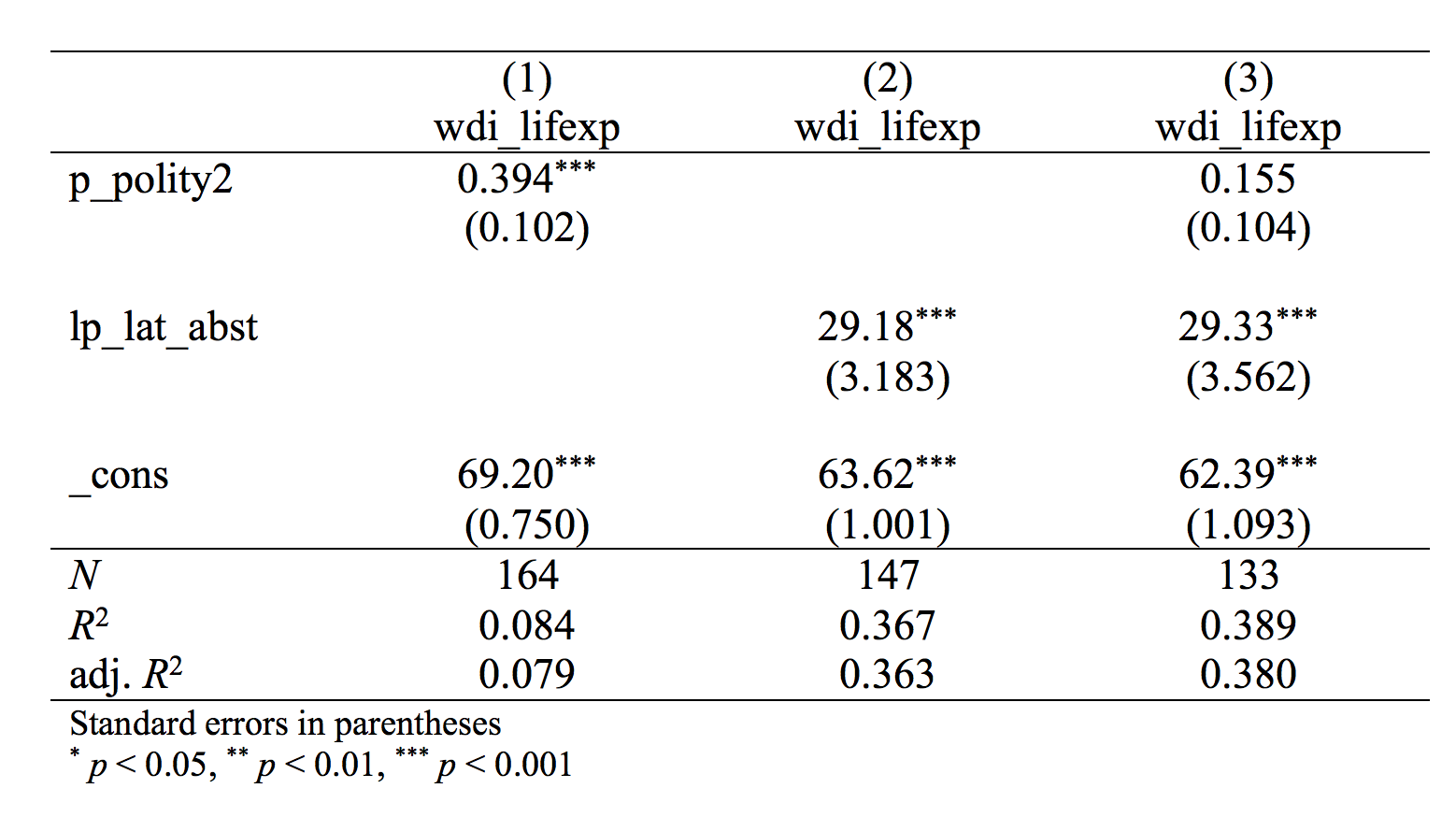
Much better! Each column represents one analysis - a "model." At the top we have what was the dependent variable in the analysis. The numbers represent the b-coefficients for each variable. In the parentheses are the t-values, and at the bottom we have the n, the number of observations.

We can see that in the first model, there was a significant relationship between democracy and life expectancy - each step up on the democracy scale is associated with an increase of life expectancy of 0.394 years. But we also see, in model 2, that countries that are further away from the equator have higher life expectancy. And we know (even though it is not evident from the table) that countries further away from the equator are more democratic. So when we control for the distance to the equator, in model 3, the coefficient for democracy is more than halved, to 0.155, and it is no longer significiant (as there are no stars next to the coefficient, and the t-value is below 1.96).

But there are other things we would like to see in the table, for instance the R²-value, or adjusted R². And we might be more interested in the standard error, rather than the t-value. Then we can add options to our command. You choose yourself what you want. Use help esttab to see the complete list of options.

esttab m1 m2 m3, se r2 ar2

------------------------------------------------------------
                      (1)             (2)             (3)   
               wdi_lifexp      wdi_lifexp      wdi_lifexp   
------------------------------------------------------------
p_polity2           0.394***                        0.155   
                  (0.102)                         (0.104)   

lp_lat_abst                         29.18***        29.33***
                                  (3.183)         (3.562)   

_cons               69.20***        63.62***        62.39***
                  (0.750)         (1.001)         (1.093)   
------------------------------------------------------------
N                     164             147             133   
R-sq                0.084           0.367           0.389   
adj. R-sq           0.079           0.363           0.380   
------------------------------------------------------------
Standard errors in parentheses
* p<0.05, ** p<0.01, *** p<0.001

This table is easy to overlook and read. The only problem is that it is not easily transferred to a Word document. If you do, you have to set the font to Courier or something else where all the letters have equal size, or all numbers will end up in the wrong places.

But a better way is to export the table to a separate file that is adapted to Word, for instance. Then you can open the file and copy the table from there to your own report.

To export the file we add using "filename.rtf" in the code. The file will then be saved in the active folder. You pick the active folder by writing cd "Users/mycomputer/statisticalanalysis/" for instance. I also add replace as an option, which means that if there is already a file with this name, it will be replaced.

esttab m1 m2 m3 using "regressiontabell.rtf", se r2 ar2 replace

(output written to regressiontabell.rtf)

If you then open the file with Word it will look like this:

You can then of course make the table even more pedagogical by replacing the variable names to more explanatory labels, for instance "Democracy (-10 to +10)" or something similar. but thist able is still a big improvement compared to the raw output.

Conclusion

To do tables with esttab thus requires three steps. First you do the analysis, then you save the results from it with estimates store and then you present the results with esttab.

Remember to always be clear and as pedagogical as possible. The person with the most to lose from the reader not understanding your results is you!